Allometric Methods
Testing allometric methods
Project Leader: Noé de la Sancha
Allometry has been used in the context of three different phenomena; ontogenetic, static, and in evolutionary allometry (Cock 1966, Cheverud 1982, Klingenberg 1996, Schlichting and Piggliucci 1998). Ontogenetic allometry refers to the growth trajectory of structures as a function of body size during the life of an individual. Static allometry refers to the scaling relationship among individuals between one structure as a function of total body size or between two structures once growth has stopped or at a particular developmental stage (Stern and Emien 1999). Meanwhile, evolutionary (phylogenetic) allometry refers to the size relationship between structures across species (Stern and Emien 1999). While the main application of allometric equations was used on morphology, virtually any feature of an organism (e.g., life history traits) can be compared to size (Stern and Emien 1999) and show simple log-log (power function) allometric scaling laws as a function of size including for example metabolic rates, lifespans, growth rates, heart rates, length and radii of aortas, cerebral gray matter, genome length, densities of mitochondria and metabolic enzymes, population density decreases (West and Brown 2005).
Bivariate approaches to allometry were represented by plotting two metric traits (usually log transformed) against each other (Huxley 1932) or by plotting a metric of shape as a function of size (Gould 1966). Bivariate techniques usually use a simple power law (West and Brown 2005) and these can take different regression approaches for example least-square regression or reduced major axis regression (Giannini et al. 2004). In these approaches significance of variables is indicative of allometry, where measures of slope (b) < 1 represent “negative” allometry and b > 1 represent “positive” allometry, while non-significant relationships represent isometry. Power functions are most commonly used and applied, but are there other functions which might be better predictors across taxa? There might be other functions beyond the power function which best explains the relationships between variables as a function of allometry and that have biological significance. There are a plethora of other potential models which might be useful in explaining these relationships. The literature for species-area relationships to explain species richness is vast with potential, meaningful models (Triantis et al. 2012, Matthews et al. 2016). Traditionally these relationships have also been assumed to be best represented by a power function. Recently, at least 20 different models have been proposed to test these relationships (Table 1). Here, we take advantage of these same models and apply them to allometric relationships of a traditional question in paleontology, biogeography, and ecology: the mass versus length relationship.
The aim of this study is to test the universality of the power function as it relates allometries of body size to other valuable life history traits. Thus we will use a dataset from across the mammal tree of life to test the 1) best fit models for body size and total length; 2) the best fit model family; 3) the best fit shape (are there asymptotes); 4) the parameters and implementation of of a power function in cases that it applies.
Methods
Data. We compiled a dataset across the mammal tree of life to test various functions to test allometries in mammals using the FuTRES datastore. We added a higher taxonomy to the dataset. MAB performed the first round of data cleaning using a simple outlier detection test. Using Noé’s expertise, he removed obvious outliers from the dataset.
Majority of these samples come from VertNet (downloaded Aug 2020 with Traiter trait extraction) which were ingested into the FuTRES datastore.
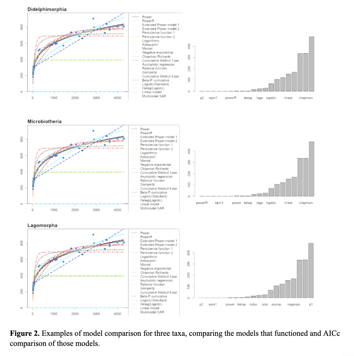
Sampling. We currently have a dataset which includes most terrestrial mammals orders. We ran preliminary data for several orders (see Figure 2) which shows the comparison of 20 mass by length functions using the sars R package (Matthews et al. 2019). Comparison via AICc shows that with these datasets the regular power function alone is not the best fit function.
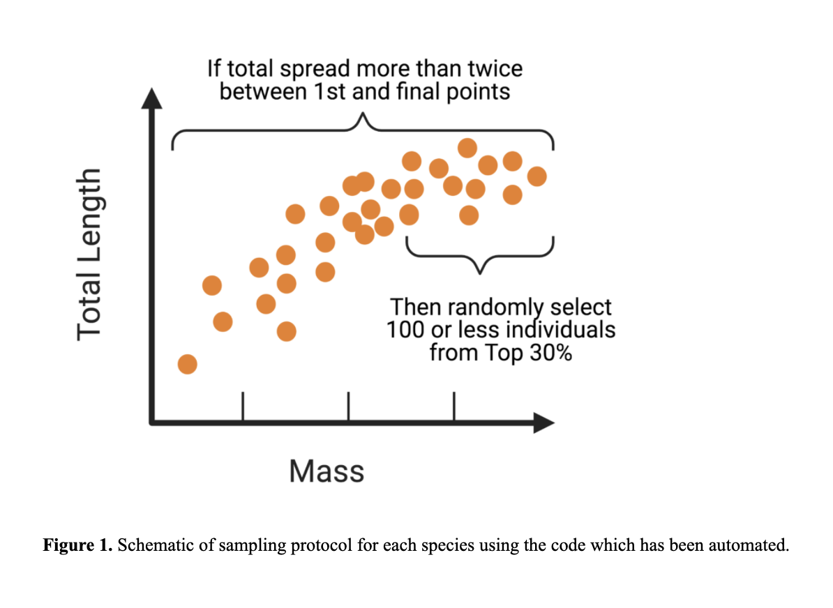
Small mammal datasets did not work at first and this was because small mammal datasets varied considerably in sample sizes per species, (ranging from a few dozens to thousands of specimens for other species), and many species clearly included juveniles to very large adults. These would be valuable to compare these at the species level but are not helpful when comparing between taxa or at the order level. Thus we began by manually curating datasets. We began by visually subsetting the ~ 30% of samples from species specific datasets (see Figure 1). After months of screening species by species by eye, Meghan developed a script to automate the dataset subsetting. We are currently in the process of testing these subsets for small mammals. We would like to run the analyses at multiple taxonomic scales, ranging from all mammals, to orders, to families, and even genera for diverse groups. We can also test this with species that have large datasets ( > 1000 specimens). We recently subsetted rodents and bats.
Analyses. We perform model selection using AICc on 20 models (Table 1). Our aim is to test the universality of mass x length relationships. We feel this is a good review to verify if the power function truly is the best approach for other taxa or datasets. And perhaps each dataset should consider comparison of these models prior to predictive analyses. FuTRES engagement
This project explicitly uses data available in the FuTRES datastore that is not available anywhere else, and is the largest specimen-level trait datastore. This project will also benefit from the technical and broad knowledge of the FuTRES community.
| No. | Fucntion name | Family | No. of parameters | Formula | Shape |
|---|---|---|---|---|---|
| 1 | Linear | Lin(A) | 2 | S = c + zA | Linear |
| 2 | Power | Pow(B) | 2 | S = cAz | Convex |
| 3 | Power_Rosenzweig | Pow(B) | 3 | S= k + cAz | Convex |
| 4 | Extended_Power_1 | Pow(B) | 3 | S = cAzA-d | Both |
| 5 | Extended_Power_2 | Pow(B) | 3 | S = cAz-(d/A) | Sigmoid |
| 6 | Persistence_Function1 | Pow(B) | 3 | S = cAz exp( - dA) | Convex |
| 7 | Persistence_Function2 | Pow(B) | 3 | S = cAz exp( - d/A) | Sigmoid |
| 8 | Exponential | Expo(C) | 2 | S = c + zlogA | Convex |
| 9 | Kobayashi_Logarithmic | Expo(C) | 2 | S = c log(1 + A/z) | Convex |
| 10 | Monod | Logis(D) | 2 | S = d /(1 + cA -1) | Convex |
| 11 | Morgan–Mercer–Flodin | Logis(D) | 3 | S = d /(1 + cA - z) | Sigmoid |
| 12 | Logistic | Logis(D) | 3 | S = c /(f + A - z) | Sigmoid |
| 13 | Negative_Exponential | Weib(E) | 2 | S = d [1 - exp( - zA)] | Convex |
| 14 | Chapman–Richards | Weib(E) | 3 | S = d [1 - exp( - zA)]c | Sigmoid |
| 15 | Weibull - 3 | Weib(E) | 3 | S = d [1 - exp( - cAz)] | Sigmoid |
| 16 | Weibull - 4 | Weib(E) | 4 | S = d [1 - exp(1cAz)]d | Sigmoid |
| 17 | Asymptotic | Asym(F) | 3 | S = d - czA | Convex |
| 18 | Rational | Rat(G) | 3 | S= (c + zA)/(1 + dA) | Convex |
| 19 | Gompertz | Gom(H) | 3 | S = d exp[ - exp( - z(A - c))] | Sigmoid |
| 20 | Beta - P | Beta(I) | 4 | S = d [1 - (1 + (A/c)z) - f] | Sigmoid |
| Roles/Competency | Identified team members | Needed team members |
|---|---|---|
| Data cleaning | Balk, de la Sancha | |
| Mammal expertise | de la Sancha | |
| R coding | Balk | more help wanted |
| Allomtery knowldege | de la Sancha | more help wanted |
| Stats knowledge for testing moedls | ||
| Partitioning small mammals | de la Sancha, Balk | more help wanted |
| Split up writing and editing assignments |